Working with Data and Models From the Literature

A very incomplete set of data from from the literature exist in $ARES/input/litdata. Each file, named using the convention <last name of first author><year>.py, is composed of dictionaries containing the information most useful to ARES (at least when first transcribed).

NOTE: May be worth interfacing with CoReCon at some point!

To see a complete listing of options, consult the following list:

%pylab inline
import ares
import numpy as np
import matplotlib.pyplot as pl

Populating the interactive namespace from numpy and matplotlib

ares.util.lit_options

['ueda2003',
 'mirocha2016',
 'test_schaerer2002',
 'song2016',
 'whitaker2012',
 'blue_tides',
 'atek2015',
 'mortlock2011',
 'bouwens2017',
 'sazonov2004',
 'dunne2009',
 'parsec',
 'eldridge2009',
 'furlanetto2017',
 'mirocha2017',
 'finkelstein2012',
 'noeske2007',
 'leitherer1999',
 'alavi2016',
 'haardt2012',
 'tomczak2014',
 'feulner2005',
 'bpass_v1',
 'aird2015',
 'mirocha2018',
 'marchesini2009_10',
 'emma',
 'vanderburg2010',
 'mirocha2019',
 'duncan2014',
 'daddi2007',
 'starburst99',
 'park2019',
 'oesch2014',
 'eldridge2017',
 'bowler2020',
 'calzetti1994',
 'oesch2013',
 'sanders2015',
 'kajisawa2010',
 'lee2011',
 'stefanon2017',
 'stark2011',
 'mcbride2009',
 'madau2014',
 'parsa2016',
 'stark2010',
 'oesch2016',
 'morishita2018',
 'perez2008',
 'ferland1980',
 'bpass_v2',
 'bowman2018',
 'sun2020',
 'gruppioni2020',
 'rojasruiz2020',
 'stefanon2019',
 'kusakabe2020',
 'finkelstein2015',
 'moustakas2013',
 'bouwens2015',
 'mirocha2020',
 'reddy2009',
 'mclure2013',
 'robertson2015',
 'mesinger2016',
 'kroupa2001',
 'karim2011',
 'schneider',
 'behroozi2013',
 'schaerer2002',
 'weisz2014',
 'oesch2018',
 'gonzalez2012',
 'inoue2011',
 'bouwens2014',
 'ueda2014']

If any of these papers ring a bell, you can check out the contents in the following way:

litdata = ares.util.read_lit('mirocha2017')  # a self-serving example

or, look directly at the source code, which lives in $ARES/input/litdata. Hopefully the contents of these files are fairly self-explanatory!

We’ll cover a few options below that I’ve used often enough to warrant the development of special routines to interface with the data and/or to plot the results nicely.

The high-z galaxy luminosity function

Measured luminosity functions from the following works are included in ARES:

• Bouwens et al. (2015)

• Finkelstein et al. (2015)

• Parsa et al. (2016)

• van der Burg et al. (2010)

• … many more now

Stellar population models

Currently, ARES can easily handle both the starburst99 original dataset and the BPASS version 1.0 models (both of which are downloaded automatically). You can access the data via

s99 = ares.util.read_lit('leitherer1999')
bpass = ares.util.read_lit('eldridge2009')

or, to create more useful objects for handling these data

s99 = ares.sources.SynthesisModel(source_sed='leitherer1999')
bpass = ares.sources.SynthesisModel(source_sed='eldridge2009')

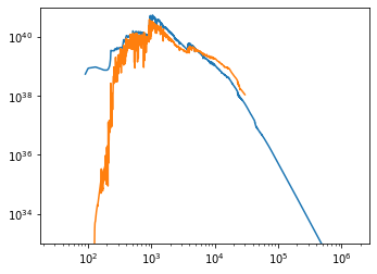
The spectra for these models are stored in the exact same way to facilitate comparison and uniform use throughout ARES. The most important attributes are wavelengths (or energies or frequencies), times, and data (a 2-D array with shape (wavelengths, times)). So, to compare the spectra for continuous star formation in the steady-state limit (ARES assumes continuous star formation by default), you could do:

pl.loglog(s99.wavelengths, s99.data[:,-1])
pl.loglog(bpass.wavelengths, bpass.data[:,-1])
pl.ylim(1e33, 1e41)

# Loaded fig8b.dat
# Loaded $ARES/input/bpass_v1/SEDS/sed.bpass.constant.nocont.sin.z020

(1e+33, 1e+41)

The most common options for these models are: pop_Z, pop_ssp, pop_binaries, pop_imf, and pop_nebular. See :doc:params_populations for a description of each of these parameters.

Parametric SEDs for galaxies and quasars

So far, there is only one litdata module in this category: the multi-wavelength AGN template described in Sazonov et al. 2004.

Reproducing Models from ARES Papers

If you’re interested in reproducing a model from a paper exactly, you can either (1) contact me directly for the model of interest, or preferably (someday) download it from my website, or (2) re-compute it yourself. In the latter case, you just need to make sure you supply the required parameters. To facilitate this, I store “parameter files” (just dictionaries) in the litdata framework as well. You can access them like any other dataset from the literature, e.g.,

m17 = ares.util.read_lit('mirocha2017')

A few of the models we focused on most get their own dictionary, for example our reference double power law model for the star-formation efficiency is stored in the dpl variable:

sim = ares.simulations.Global21cm(**m17.dpl)
sim.run()
sim.GlobalSignature()  # voila!

# Loaded $ARES/input/inits/inits_planck_TTTEEE_lowl_lowE_best.txt.

############################################################################
##                       ARES Simulation: Overview                        ##
############################################################################
## ---------------------------------------------------------------------- ##
## Source Populations                                                     ##
## ---------------------------------------------------------------------- ##
##           sfrd    sed  radio  O/IR  Lya    LW   LyC   Xray  RTE        ##
## pop #0 : sfe-func  yes    -     -     x     x     x     -     x        ##
## pop #1 : sfrd->0   yes    -     -     -     -     -     x     x        ##
## ---------------------------------------------------------------------- ##
## Notes                                                                  ##
## ---------------------------------------------------------------------- ##
## + pop_calib_lum != None, which means changes to pop_Z                  ##
##   will *not* affect UVLF. Set pop_calib_lum=None to restore            ##
##   "normal" behavior (see S3.4 in Mirocha et al. 2017).                 ##
## ---------------------------------------------------------------------- ##
## Physics                                                                ##
## ---------------------------------------------------------------------- ##
## cgm_initial_temperature        : 20000                                 ##
## clumping_factor                : 3                                     ##
## secondary_ionization           : 3                                     ##
## approx_Salpha                  : 3                                     ##
## include_He                     : True                                  ##
## feedback_LW                    : False                                 ##
############################################################################
# Loaded $ARES/input/bpass_v1/SEDS/sed.bpass.constant.nocont.sin.z020
# WARNING: revisit scalability wrt fesc.
# Loaded $ARES/input/hmf/hmf_ST_planck_TTTEEE_lowl_lowE_best_logM_1400_4-18_z_1201_0-60.hdf5.
# Loaded /Users/jordanmirocha/Dropbox/work/mods/ares/input/optical_depth/optical_depth_planck_TTTEEE_lowl_lowE_best_He_1000x2158_z_5-60_logE_2.3-4.5.hdf5.

gs-21cm: 100% |#############################################| Time:  0:00:03

(<AxesSubplot:xlabel='$\\nu \\ (\\mathrm{MHz})$', ylabel='$\\delta T_b \\ (\\mathrm{mK})$'>,
 <AxesSubplot:label='3dcb6a54-8157-4a42-875a-4e57501414d7', xlabel='$z$'>)

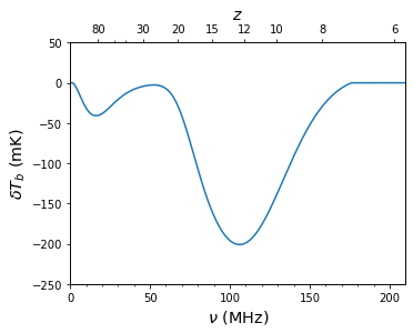
Hopefully this results exactly in the solid black curve from Figure 2 of Mirocha, Furlanetto, & Sun (2017) <http://adsabs.harvard.edu/abs/2017MNRAS.464.1365M>_, provided you’re using ARES version 0.2. If it doesn’t, please contact me.

NOTE: If using a newer version of the code, this may shift slightly due to changes in the default cosmological parameters and halo mass function. If you pull a recent version and the result is significantly different, please get in touch with me.

Alternatively, you can use the ParameterBundle framework, which also taps into our collection of data from the literature. To access the set of parameters for the “dpl” model, you simply do:

pars = ares.util.ParameterBundle('mirocha2017:dpl')

This tells ARES to retrieve the dpl variable within the mirocha2017 module. See :doc:param_bundles for more on these objects.

Mirocha, Furlanetto, & Sun (2017) (mirocha2017)

This model has a few options: dpl, and the extensions floor and steep, as explored in the paper.

Non-standard pre-requisites: * High resolution optical depth table for X-ray background. To generate one for yourself, navigate to $ARES/input/optical_depth and open the generate_optical_depth_tables.py file. Between lines 35 and 45 there are a block of parameters that set the resolution of the table. Make sure that helium=1, zi=50, zf=5, and Nz=[1e3]. It should only take a few minutes to generate this table.

The following parameters are uncertain and typically treated as free parameters within the ranges denoted by brackets (not all of which are hard limits):

* ``pop_Z{0}``, :math:`[0.001, 0.04]`
* ``pop_Tmin{0}``, :math:`[300, \sim \mathrm{few} \times 10^5]`  (``pop_Tmin{1}`` is tied to this value by default).
* ``pop_fesc{0}``, in general can lie in range :math:`[0, 1]`, but for consistency with observational constraints on :math:`\tau_e` (from, e.g., *Planck*), it's probably best to limit values to :math:`\lesssim 0.2`.
* ``pop_fesc_LW{0}``, :math:`[0, 1]`
* ``pop_rad_yield{1}``, :math:`[10^{38}, 10^{42}]` :math:`2.6 \times 10^{39}` by default
* ``pop_logN{1}``, :math:`[18, 23]`, :math:`-\infty` by default.

NOTE: Changes in the metallicity (pop_Z{0}) in general affect the luminosity function (LF). However, by default, the normalization of the star formation efficiency will automatically be adjusted to guarantee that the LF does not change upon changes to pop_Z{0}. Set the pop_calib_lum{0} parameter to None to remove this behavior.

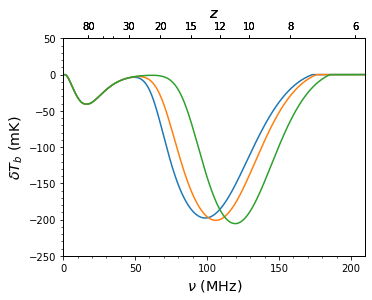
To re-make the right-hand panel of Figure 1 from the paper, you could do something like:

dpl = ares.util.ParameterBundle('mirocha2017:dpl')

ax = None
for model in ['floor', 'dpl', 'steep']:
    pars = dpl + ares.util.ParameterBundle('mirocha2017:%s' % model)
    sim = ares.simulations.Global21cm(verbose=False, progress_bar=False, **pars)
    sim.run()
    ax, zax = sim.GlobalSignature(ax=ax)

# WARNING: revisit scalability wrt fesc.
# WARNING: revisit scalability wrt fesc.
# WARNING: revisit scalability wrt fesc.

For more thorough parameter space explorations, you might want to consider using the ModelGrid (see the example or ModelSample (:doc:example_mc_sampling) machinery. If you’d like to do some forecasting or fitting with these models, check out :doc:example_mcmc_gs and :doc:example_mcmc_lf.

NOTE: Notice that the floor and steep options are defined relative to the dpl model, i.e., they only contain the parameters that are different from the dpl model, which is why we updated the parameter dictionary rather than creating a new one just with the steep or floor parameters.

Furlanetto et al. (2017) (furlanetto2017)

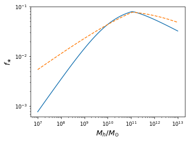
The main options in this model are whether to use momentum-driven or energy-driven feedback, what are accessible separately via, e.g.,

E = ares.util.ParameterBundle('furlanetto2017:energy')
p = ares.util.ParameterBundle('furlanetto2017:momentum')
fshock = ares.util.ParameterBundle('furlanetto2017:fshock')

The only difference is the assumed slope of the star formation efficiency in low-mass halos, which is defined in the parameter 'pq_func_par2[0]', i.e., the third parameter (par2) of the first parameterized quantity ([0]), in addition to a power-law index that describes the rate of redshift evolution, pq_func_par2[1].

To do a quick comparison, you could simply do:

import ares

ls = ['-', '--']
for i, model in enumerate([E, p]):
    pars = model + fshock
    pop = ares.populations.GalaxyPopulation(**pars)
    M = np.logspace(7, 13)
    pl.loglog(M, pop.fstar(z=6, Mh=M), ls=ls[i])

pl.xlabel(r'$M_h / M_{\odot}$')
pl.ylabel(r'$f_{\ast}$')

Text(0, 0.5, '$f_{\\ast}$')

Creating your own

As with parameter bundles, you can write your own litdata modules without modifying the ARES source code. Just create a new .py file and stick it in one of the following places (searched in this order!):

• Your current working directory.

• $HOME/.ares

• $ARES/input/litdata

For example, if I created the following file (junk_lf.py; which you’ll notice resembles the other LF litdata modules) in my current directory:

redshifts = [4, 5]
wavelength = 1600.
units = {'phi': 1}  # i.e., not abundances not recorded as log10 values

data = {}
data['lf'] = \
{
 4: {
     'M': [-23, -22, -21, -20],
     'phi': list(np.random.rand(4) * 1e-4),
     'err': [tuple(np.random.rand(2) * 1e-7) for i in range(4)]
    },
 5: {
     'M': [-23, -22, -21, -20],
     'phi': list(np.random.rand(4) * 1e-4),
     'err': [tuple(np.random.rand(2) * 1e-7) for i in range(4)],
    }
}

then the built-in plotting routines will automatically find it. For example, you could compare this completely made-up LF with the rest via the commands obslf = ares.analysis.GalaxyPopulation(); ax = obslf.Plot(z=4, sources='junk_lf').