Self-Consistent Dust Reddening
In Mirocha, Mason, & Stark (2020), we describe a simple extension to the now-standard galaxy model in ARES that generates ultraviolet colours self-consistently, rather than invoking IRX-\(\beta\) relations to perform a dust correction. Here, we describe how to work with these new models.
Preliminaries
Before getting started, two lookup tables are required that don’t ship by default with ARES (via the remote.py script; see ARES installation):
A new halo mass function lookup table that employs the Tinker et al. 2010 results, rather than Sheth-Tormen (used in most earlier work with ARES).
A lookup table of halo mass assembly histories.
To create these yourself, you’ll need the hmf code, which is installable via pip.
This should only take a few minutes even in serial. First, navigate to $ARES/input/hmf, where you should see a few .hdf5 files and Python scripts. Open the file generate_hmf_tables.py and make the following adjustments to the parameter dictionary:
[1]:
def_kwargs = \
{
 "hmf_model": 'Tinker10',

 "hmf_tmin": 30,
 "hmf_tmax": 2e3,
 "hmf_dt": 1,

 "cosmology_id": 'paul',
 "cosmology_name": 'user',
 "sigma_8": 0.8159,
 'primordial_index': 0.9652,
 'omega_m_0': 0.315579,
 'omega_b_0': 0.0491,
 'hubble_0': 0.6726,
 'omega_l_0': 1. - 0.315579,
}
The new HMF table will use constant 1 Myr time-steps, rather than the default redshift steps, and employ a cosmology designed to remain consistent with another project (led by a collaborator whose name you can probably guess)!
Once you’ve run the generate_hmf_tables.py script, you should have a new file, hmf_Tinker10_user_paul_logM_1400_4-18_t_1971_30-2000.hdf5, sitting inside $ARES/input/hmf. Now, we’re almost done. Simply execute:
python generate_halo_histories.py hmf_Tinker10_user_paul_logM_1400_4-18_t_1971_30-2000.hdf5
The additional resulting file, hgh_Tinker10_user_paul_logM_1400_4-18_t_1971_30-2000_xM_10_0.10.hdf5, will be found automatically in subsequent calculations.
Example
With the required lookup tables now in hand, we can start in the usual way:
[2]:
%pylab inline
import ares
import numpy as np
import matplotlib.pyplot as pl
Populating the interactive namespace from numpy and matplotlib
and read-in the best-fit parameters via
[3]:
pars = ares.util.ParameterBundle('mirocha2020:univ')
Now, we create a GalaxyPopulation object,
[4]:
pop = ares.populations.GalaxyPopulation(**pars)
which is an instance of the GalaxyEnsemble class, rather than the GalaxyCohort class, the latter of which is described in this example. This offers a more general approach, including more complex star formation histories and proper treatment of spectral synthesis.
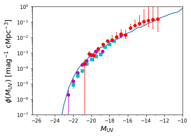
We can plot the UVLF in the usual way,
[5]:
# First, some data
obslf = ares.analysis.GalaxyPopulation()
ax = obslf.PlotLF(z=6, round_z=0.2)

# Now, the predicted/calibrated UVLF
mags = np.arange(-30, 10, 0.5)
_mags, phi = pop.LuminosityFunction(6, mags)

ax.semilogy(mags, phi)
/Users/jordanmirocha/Dropbox/work/soft/miniconda3/lib/python3.7/site-packages/numpy/ma/core.py:2826: UserWarning: Warning: converting a masked element to nan.
  order=order, subok=True, ndmin=ndmin)
/Users/jordanmirocha/Dropbox/work/soft/miniconda3/lib/python3.7/site-packages/numpy/core/_asarray.py:171: UserWarning: Warning: converting a masked element to nan.
  return array(a, dtype, copy=False, order=order, subok=True)
/Users/jordanmirocha/Dropbox/work/soft/miniconda3/lib/python3.7/site-packages/numpy/core/_asarray.py:102: UserWarning: Warning: converting a masked element to nan.
  return array(a, dtype, copy=False, order=order)
# WARNING: finkelstein2015 wavelength=1500.0A, not 1600A!
# Loaded $ARES/input/hmf/hgh_Tinker10_user_paul_logM_1400_4-18_t_1971_30-2000_xM_10_0.10.hdf5.
# Loaded $ARES/input/hmf/hmf_Tinker10_user_paul_logM_1400_4-18_t_1971_30-2000.hdf5.
# Loaded $ARES/input/bpass_v1/SEDS/sed.bpass.instant.nocont.sin.z004.deg10
[5]:
[<matplotlib.lines.Line2D at 0x1901dcdd0>]
The main difference between these models and the simpler models (from, e.g., the mirocha2017 parameter bundle) is access to UV colours. To access them, you can do, e.g.,
[6]:
filt, mags = pop.get_mags(6., presets='hst', wave=1600., )
beta = pop.get_beta(6., presets='hst')
pl.scatter(mags, beta, alpha=0.1, color='b', edgecolors='none')
l(nu): 100% |###############################################| Time:  0:00:01
l(nu): 100% |###############################################| Time:  0:00:00
[6]:
<matplotlib.collections.PathCollection at 0x1831c7590>
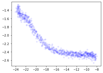
This will take order \(\simeq 10\) seconds, as modeling UV colours requires synthesizing a reasonbly high resolution (\(\Delta \lambda = 20 \unicode{x212B}\) by default) spectrum for each galaxy in the model, so that there are multiple points within photometric windows.
This example computes the UV slope \(\beta\) using the Hubble filters appropriate for the input redshift (see Table A1 in the paper).
NOTE: Other presets include 'jwst', 'jwst-w', 'jwst-m', and 'calzetti1994'.
You can bin points in the \(M_{\text{UV}}-\beta\) plane, if you prefer it, via the return_binned keyword argument,
[7]:
# Plot scatter in each MUV bin as errorbars
mags = np.arange(-25, -10, 0.5) # bin centers
beta, beta_s = pop.get_beta(6., presets='hst', Mbins=mags, return_binned=True,
    return_scatter=True)

pl.errorbar(mags, beta, yerr=beta_s.T, color='b', marker='s', fmt='o')
l(nu): 100% |###############################################| Time: 0:00:00
[7]:
<ErrorbarContainer object of 3 artists>
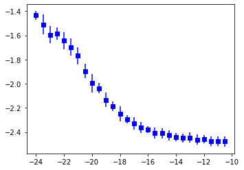
NOTE: Computing colors from fits in the Calzetti et al. 1994 windows requires higher spectral resolution, given that these windows are each only \(\Delta \lambda \sim 10 \unicode{x212B}\) wide. Adjust the dlam keyword argument to increase the wavelength-sampling used prior to photometric UV slope estimation.
Lastly, to extract the “raw” galaxy population properties, like SFR, stellar mass, etc., you can use the get_field method, e.g.,
[8]:
Ms = pop.get_field(6., 'Ms') # stellar mass
Md = pop.get_field(6., 'Md') # dust mass
Sd = pop.get_field(6., 'Sd') # dust surface density
# etc.
To see what’s available, check out
[9]:
pop.histories.keys()
[9]:
dict_keys(['nh', 'Mh', 'MAR', 't', 'z', 'children', 'zthin', 'SFR', 'Ms', 'MZ', 'Md', 'Sd', 'fcov', 'Mg', 'Z', 'bursty', 'pos', 'Nsn', 'rand'])
From these simple commands, most plots and analyses from the paper can be reproduced in relatively short order.
Notes on performance
The compute time for these models is determined largely by three factors:
The number of halos (really halo bins) we evolve forward in time. The default
mirocha2020:univmodels use \(\Delta \log_{10} M_h = 0.01\) mass-bins, each with 10 halos (pop_thin_hist=10). For a larger sample, e.g., when lots of scatter is being employed, larger values ofpop_thin_histmay be warranted.The number of observed redshifts at which \(\beta\) is synthesize, since new spectra must be generated.
The number of wavelengths used to sample the intrinsic UV spectrum of galaxies. When computing \(\beta\) via photometry (Hubble or JWST), \(\Delta \lambda = 20 \unicode{x212B}\) will generally suffice.
For the models in Mirocha, Mason, & Stark (2020), with \(\Delta \log_{10} M_h = 0.01\) (hmf_logM=0.01), pop_thin_hist=10, calibrating at two redshifts for \(\beta\) (4 and 6), with \(\Delta \lambda = 20 \unicode{x212B}\), each model takes \(\sim 10-20\) seconds, depending on your machine.
NOTE: Generating the UVLF is essentially free compared to computing \(\beta\).
For more information on what’s happening under the hood, e.g., with regards to spectral synthesis and noisy star-formation histories, see Example: spectral synthesis.
[ ]:
[ ]: