More Realistic Galaxy Populations

Most global 21-cm examples in the documentation tie the volume-averaged emissivity of galaxies to the rate at which mass collapses into dark matter halos (this is the default option in ARES). Because of this, they are referred to as \(f_{\text{coll}}\) models throughout, and are selected by setting pop_sfr_model='fcoll'. In the code, they are represented by GalaxyAggregate objects, named as such because galaxies are only modeled in aggregate, i.e., there is no distinction in the properties of galaxies as a function of mass, luminosity, etc.

However, we can also run more detailed models in which the properties of galaxies are allowed to change as a function of halo mass, redshift, and/or potentially other quantities.

A few usual imports before we begin:

%pylab inline
import ares
import numpy as np
import matplotlib.pyplot as pl

Populating the interactive namespace from numpy and matplotlib

Double Power-Law Star Formation Efficiency

The most common extension to simple models is to allow the star formation efficiency (SFE) to vary as a function of halo mass. This is motivated observationally by the mismatch in the shape of the galaxy luminosity function (LF) and dark matter halo mass function (HMF). In Mirocha, Furlanetto, & Sun (2017), we adopted a double power-law form for the SFE, i.e.,

\begin{equation} f_{\ast}(M_h) = \frac{2 f_{\ast,p}} {\left(\frac{M_h}{M_{\text{p}}} \right)^{\gamma_{\text{lo}}} + \left(\frac{M_h}{M_{\text{p}}} \right)^{\gamma_{\text{hi}}}} \end{equation}

where the free parameters are the normalization, \(f_{\ast,p}\), the peak mass, \(M_p\), and the power-law indices in the low-mass and high-mass limits, \(\gamma_{\text{lo}}\) and \(\gamma_{\text{hi}}\), respectively. Combined with a model for the mass accretion rate onto dark matter halos (\(\dot{M}_h\); see next section), the star formation rate as computed as

\begin{equation} \dot{M}_{\ast} = f_{\ast} \left(\frac{\Omega_{b,0}}{\Omega_{m,0}} \right) \dot{M}_h \end{equation}

In general, the SFE curve must be calibrated to an observational dataset (see Fitting to UVLFs), but you can also just grab our best-fitting parameters for a redshift-independent SFE curve as follows:

p = ares.util.ParameterBundle('mirocha2017:base')
pars = p.pars_by_pop(0, strip_id=True)

The second command extracts only the parameters associated with population #0, which is the stellar population in this calculation (population #1 is responsible for X-ray emission only; see Models with Multiple Source Populations for more info on the approach to populations in ARES). Passing strip_id=True removes all ID numbers from parameter names, e.g., pop_sfr_model{0} becomes pop_sfr_model. The reason for doing that is so we can generate a single GalaxyPopulation instance, e.g.,

pop = ares.populations.GalaxyPopulation(**pars)

If you glance at the contents of pars, you’ll notice that the parameters that define the double power-law share a pq prefix. This is short for “parameterized quantity”, and is discussed more generally on the page about the ParameterizedQuantity object.

NOTE: You can access population objects used in a simulation via the pops attribute, which is a list of population objects that belongs to instances of common simulation classes like Global21cm, MetaGalacticBackground, etc.

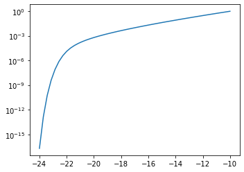
Now, to generate a model for the luminosity function, simply define your redshift of interest and array of magnitudes (assumed to be rest-frame \(1600 \unicode{x212B}\) AB magnitudes), and pass them to the aptly named LuminosityFunction function,

z = 6
MUV = np.linspace(-24, -10)
_bins, lf = pop.get_lf(z, MUV)

pl.semilogy(MUV, lf)

# Loaded $ARES/input/hmf/hmf_ST_planck_TTTEEE_lowl_lowE_best_logM_1400_4-18_z_1201_0-60.hdf5.
# Loaded $ARES/input/bpass_v1/SEDS/sed.bpass.constant.nocont.sin.z020

[<matplotlib.lines.Line2D at 0x10d6fac90>]

To compare to the observed galaxy luminosity function, we can use some convenience routines setup to easily access and plot measurements stored in the ARES litdata module:

obslf = ares.analysis.GalaxyPopulation()
ax = obslf.Plot(z=z, round_z=0.2)
ax.semilogy(MUV, lf)
ax.set_ylim(1e-8, 10)
ax.legend()

/Users/jordanmirocha/Dropbox/work/soft/miniconda3/lib/python3.7/site-packages/numpy/ma/core.py:2826: UserWarning: Warning: converting a masked element to nan.
  order=order, subok=True, ndmin=ndmin)
/Users/jordanmirocha/Dropbox/work/soft/miniconda3/lib/python3.7/site-packages/numpy/core/_asarray.py:171: UserWarning: Warning: converting a masked element to nan.
  return array(a, dtype, copy=False, order=order, subok=True)
/Users/jordanmirocha/Dropbox/work/soft/miniconda3/lib/python3.7/site-packages/numpy/core/_asarray.py:102: UserWarning: Warning: converting a masked element to nan.
  return array(a, dtype, copy=False, order=order)

# WARNING: finkelstein2015 wavelength=1500.0A, not 1600.0A!

<matplotlib.legend.Legend at 0x18f924510>

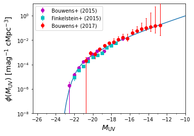
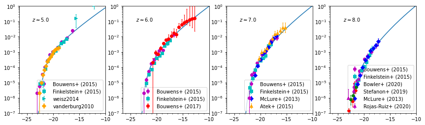
The round_z keyword argument makes it so that any dataset available in the range \(5.8 \leq z \leq 6.2\) gets included in the plot. To do this for multiple redshifts at the same time, you could do something like:

redshifts = [5,6,7,8]
MUV = np.linspace(-24, -10)


# Create a 1x4 panel plot, include all available data sources
fig, axes = pl.subplots(1, len(redshifts), figsize=(4*len(redshifts), 4))

for i, z in enumerate(redshifts):
    obslf.Plot(z=z, round_z=0.3, ax=axes[i])

    _bins, lf = pop.get_lf(z, MUV)
    axes[i].semilogy(MUV, lf)
    axes[i].annotate(r'$z \simeq %.1f$' % z, (-24, 1e-1))
    axes[i].legend(loc='lower right')

/Users/jordanmirocha/Dropbox/work/soft/miniconda3/lib/python3.7/site-packages/numpy/ma/core.py:2826: UserWarning: Warning: converting a masked element to nan.
  order=order, subok=True, ndmin=ndmin)
/Users/jordanmirocha/Dropbox/work/soft/miniconda3/lib/python3.7/site-packages/numpy/core/_asarray.py:171: UserWarning: Warning: converting a masked element to nan.
  return array(a, dtype, copy=False, order=order, subok=True)
/Users/jordanmirocha/Dropbox/work/soft/miniconda3/lib/python3.7/site-packages/numpy/core/_asarray.py:102: UserWarning: Warning: converting a masked element to nan.
  return array(a, dtype, copy=False, order=order)

# WARNING: finkelstein2015 wavelength=1500.0A, not 1600.0A!
# WARNING: weisz2014 wavelength=1700.0A, not 1600.0A!
# WARNING: vanderburg2010 wavelength=1500.0A, not 1600.0A!

/Users/jordanmirocha/Dropbox/work/soft/miniconda3/lib/python3.7/site-packages/numpy/ma/core.py:2826: UserWarning: Warning: converting a masked element to nan.
  order=order, subok=True, ndmin=ndmin)
/Users/jordanmirocha/Dropbox/work/soft/miniconda3/lib/python3.7/site-packages/numpy/core/_asarray.py:171: UserWarning: Warning: converting a masked element to nan.
  return array(a, dtype, copy=False, order=order, subok=True)
/Users/jordanmirocha/Dropbox/work/soft/miniconda3/lib/python3.7/site-packages/numpy/core/_asarray.py:102: UserWarning: Warning: converting a masked element to nan.
  return array(a, dtype, copy=False, order=order)

# WARNING: finkelstein2015 wavelength=1500.0A, not 1600.0A!

/Users/jordanmirocha/Dropbox/work/soft/miniconda3/lib/python3.7/site-packages/numpy/ma/core.py:2826: UserWarning: Warning: converting a masked element to nan.
  order=order, subok=True, ndmin=ndmin)
/Users/jordanmirocha/Dropbox/work/soft/miniconda3/lib/python3.7/site-packages/numpy/core/_asarray.py:171: UserWarning: Warning: converting a masked element to nan.
  return array(a, dtype, copy=False, order=order, subok=True)
/Users/jordanmirocha/Dropbox/work/soft/miniconda3/lib/python3.7/site-packages/numpy/core/_asarray.py:102: UserWarning: Warning: converting a masked element to nan.
  return array(a, dtype, copy=False, order=order)

# WARNING: finkelstein2015 wavelength=1500.0A, not 1600.0A!
# WARNING: mclure2013 wavelength=1500.0A, not 1600.0A!
# WARNING: atek2015 wavelength=1500.0A, not 1600.0A!

/Users/jordanmirocha/Dropbox/work/soft/miniconda3/lib/python3.7/site-packages/numpy/ma/core.py:2826: UserWarning: Warning: converting a masked element to nan.
  order=order, subok=True, ndmin=ndmin)
/Users/jordanmirocha/Dropbox/work/soft/miniconda3/lib/python3.7/site-packages/numpy/core/_asarray.py:171: UserWarning: Warning: converting a masked element to nan.
  return array(a, dtype, copy=False, order=order, subok=True)
/Users/jordanmirocha/Dropbox/work/soft/miniconda3/lib/python3.7/site-packages/numpy/core/_asarray.py:102: UserWarning: Warning: converting a masked element to nan.
  return array(a, dtype, copy=False, order=order)

# WARNING: finkelstein2015 wavelength=1500.0A, not 1600.0A!
# WARNING: bowler2020 wavelength=1500.0A, not 1600.0A!
# WARNING: stefanon2019 wavelength=1500.0A, not 1600.0A!
# WARNING: mclure2013 wavelength=1500.0A, not 1600.0A!
# WARNING: rojasruiz2020 wavelength=1500.0A, not 1600.0A!

To create the GalaxyPopulation used above from scratch (i.e., without using parameter bundles), we could have just done:

pars = \
{
 'pop_sfr_model': 'sfe-func',
 'pop_sed': 'eldridge2009',


 'pop_fstar': 'pq',
 'pq_func': 'dpl',
 'pq_func_par0': 0.05,
 'pq_func_par1': 2.8e11,
 'pq_func_par2': 0.51,
 'pq_func_par3': -0.61,
 'pq_func_par4': 1e10,  # halo mass at which SFE is normalized
}


pop = ares.populations.GalaxyPopulation(**pars)

NOTE: Beware that by default, the double power-law is normalized at \(M_h = 10^{10} \ M_{\odot}\) (see ps_func_par4 above), whereas the Equation above for \(f_{\ast}\) is defined such that pq_func_par0 refers to the SFE at the peak mass. If you prefer a peak-normalized SFE, you can set pq_func='dpl_normP' instead.

Accretion Models

By default, ARES will derive the mass accretion rate (MAR) onto halos from the HMF itself (see Section 2.2 of Furlanetto et al. 2017 for details). That is, pop_MAR='hmf' by default. There are also two other options:

• Plug-in your favorite mass accretion model as a lambda function, e.g., pop_MAR=lambda z, M: 1. * (M / 1e12)**1.1 * (1. + z)**2.5.

• Grab a model from litdata. The median MAR from McBride et al. (2009) is included (same as above equation), and can used as pop_MAR='mcbride2009'. If you’d like to add more options, use ares/input/litdata/mcbride2009.py as a guide.

WARNING: Note that the MAR formulae determined from numerical simulations may not have been calibrated at the redshifts most often targeted in ARES calculations, nor are they guaranteed to be self-consistent with the HMF used in ARES. One approach used in Sun & Furlanetto (2016) is to re-normalize the MAR by requiring its integral to match that predicted by \(f_{\text{coll}}(z)\), which can boost the accretion rate at high redshifts by a factor of few. Setting pop_MAR_conserve_norm=True will enforce this condition in ARES.

See this page for more information.