The ParameterizedQuantity Framework

The goal of this framework is to make it possible to take any parameter in ARES (the ones that take on numerical values, anyways), and convert it from a constant to a function of an arbitrary set of variables.

One approach is to allow the user to supply a function of their own to each parameter in place of a numerical value. ARES permits this functionality for some parameters (e.g., pop_sed), however, it is often advantageous to retain access to the parameters of the user-supplied function, for example to allow these parameters to vary in some fit. This is the primary motivation for the ParameterizedQuantity framework.

We have already seen PQs in use in the More Realistic Galaxy Populations example, which showed how to make the efficiency of star formation a function of halo mass:

%pylab inline
import ares
import numpy as np
import matplotlib.pyplot as pl

Populating the interactive namespace from numpy and matplotlib

pars = \
{
 'pop_sfr_model': 'sfe-func',
 'pop_sed': 'eldridge2009',

 'pop_fstar': 'pq',
 'pq_func': 'dpl',
 'pq_func_var': 'Mh',
 'pq_func_par0': 0.05,
 'pq_func_par1': 2.8e11,
 'pq_func_par2': 0.51,
 'pq_func_par3': -0.61,
 'pq_func_par4': 1e10,  # Halo mass at which fstar is normalized
}

pop = ares.populations.GalaxyPopulation(**pars)

There are three important steps shown above:

• Setting pop_fstar='pq' tells ARES that this quantity will be represented by a PQ object. With no ID number supplied, it is assumed that parameters with the prefix pq are used to construct this object.

• The function adopted is a double power-law, 'dpl', which is a four-parameter model. The parameters pq_func_par0, pq_func_par1, etc. store the values of these parameters. The meaning of the parameters is of course different depending on what function we choose – see this listing of the available functions and their corresponding parameters.

• The independent variable is halo mass, Mh. Note that this name is important, i.e., just M will cause an error. This is a convention of the :class:GalaxyCohort <ares.populations.GalaxyCohort.GalaxyCohort> class.

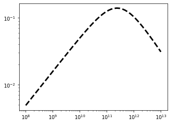
Let’s plot it just for a sanity check:

Mh = np.logspace(8, 13)
sfe_dpl = pop.fstar(z=6, Mh=Mh)

pl.loglog(Mh, sfe_dpl, color='k', ls='--', lw=3)

[<matplotlib.lines.Line2D at 0x179d95090>]

Multi-Variable ParameterizedQuantity

More complicated models are also available. For example, say we wanted to allow the normalization of the SFE to evolve with redshift, i.e.,

\[f_{\ast}(M_h) = \frac{2 f_{\ast,0} \left(\frac{1+z}{7}\right)^{\gamma_z}} {\left(\frac{M_h}{M_{\text{p}}} \right)^{\gamma_{\text{lo}}} + \left(\frac{M_h}{M_{\text{p}}} \right)^{\gamma_{\text{hi}}}}\]

Starting from the pure dpl model above, we can make a few modifications:

# Extra multiplicative boost with redshift, par0 * (var / par1)**par2
pars = \
{
 'pop_sfr_model': 'sfe-func',
 'pop_sed': 'eldridge2009',

 'pop_fstar': 'pq[0]',      # Give it an ID this time, since we'll add another
 'pq_func[0]': 'dpl_evolN', # dpl w/ evolution in the Normalization
 'pq_func_var[0]': 'Mh',
 'pq_func_var2[0]': '1+z',  # indicate 1+z as the second indep. variable

 # Old parameters that we still need
 'pq_func_par0[0]': 0.05,
 'pq_func_par1[0]': 2.8e11,
 'pq_func_par2[0]': 0.51,
 'pq_func_par3[0]': -0.61,
 'pq_func_par4[0]': 1e10,
 'pq_func_par5[0]': 7.,     # New param: "pivot" redshift
 'pq_func_par6[0]': 1.,     # New param: PL evolution index
}

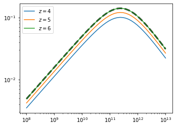
To verify that this has worked, let’s again plot the SFE, now as a function of redshift, and compare to the previous \(z\)-independent model:

pop = ares.populations.GalaxyPopulation(**pars)

redshifts = [4,5,6]
Mh = np.logspace(8, 13)

pl.loglog(Mh, sfe_dpl, color='k', ls='--', lw=3)
for z in redshifts:
    fstar = pop.SFE(z=z, Mh=Mh)
    pl.loglog(Mh, fstar, label=r'$z={}$'.format(z))

pl.legend()

<matplotlib.legend.Legend at 0x17a02f110>

NOTE: The only method of ParameterizedQuantity objects ever called is the __call__ method, which accepts **kwargs. As a result, we must always supply arguments accordingly (i.e., supplying positional arguments only will not suffice), hence the z=z, Mh=Mh usage above.

Multiple ParameterizedQuantity objects at once

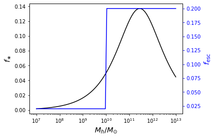
In general, we can use the same approach outlined above to parameterize other quantities as a function of halo mass and/or redshift. For example, we can use a double power-law SFE model and set the escape fraction to be a step function in halo mass,

pars = \
{
 'pop_sfr_model': 'sfe-func',
 'pop_sed': 'eldridge2009',

 'pop_fstar': 'pq[0]',
 'pq_func[0]': 'dpl',
 'pq_func_par0[0]': 0.05,
 'pq_func_par1[0]': 2.8e11,
 'pq_func_par2[0]': 0.5,
 'pq_func_par3[0]': -0.5,
 'pq_func_par4[0]': 1e10,

 'pop_fesc': 'pq[1]',
 'pq_func[1]': 'step_abs',
 'pq_func_par0[1]': 0.02,
 'pq_func_par1[1]': 0.2,
 'pq_func_par2[1]': 1e10,
}

Note that here we gave ID numbers for each PQ in square brackets, both when identifying the parameters to be treated as PQs (pop_fstar and pop_fesc) and when setting the values of their sub-parameters (e.g., pq_func[0], pq_func_par0[0], etc.

To check the result:

pop = ares.populations.GalaxyPopulation(**pars)

Mh = np.logspace(7, 13, 100)

fig, ax1 = pl.subplots(num=2)

ax1.semilogx(Mh, pop.fstar(z=6, Mh=Mh), color='k')
ax1.set_ylabel(r'$f_{\ast}$')
ax1.set_xlabel(r'$M_h / M_{\odot}$')

ax2 = ax1.twinx()
ax2.tick_params('y', colors='b')
ax2.set_ylabel(r'$f_{\mathrm{esc}}$', color='b')
ax2.semilogx(Mh, pop.fesc(z=6, Mh=Mh), color='b')

[<matplotlib.lines.Line2D at 0x17a4c8b10>]

Allowed Parameters

An incomplete list so far:

• pop_fstar

• pop_fesc

• pop_focc