Simple Physical Models for the Global 21-cm Signal

To begin, first import ares and a few standards

%pylab inline
import ares
import matplotlib.pyplot as pl

Populating the interactive namespace from numpy and matplotlib

To generate a model of the global 21-cm signal, we need to use the ares.simulations.Global21cm class. With no arguments, default parameter values will be used:

sim = ares.simulations.Global21cm()

# Loaded $ARES/input/inits/inits_planck_TTTEEE_lowl_lowE_best.txt.

############################################################################
##                       ARES Simulation: Overview                        ##
############################################################################
## ---------------------------------------------------------------------- ##
## Source Populations                                                     ##
## ---------------------------------------------------------------------- ##
##           sfrd    sed  radio  O/IR  Lya    LW   LyC   Xray  RTE        ##
## pop #0 :  fcoll    yes    -     -     x     x     -     -              ##
## pop #1 : sfrd->0   yes    -     -     -     -     -     x              ##
## pop #2 : sfrd->0   yes    -     -     -     -     x     -              ##
## ---------------------------------------------------------------------- ##
## Physics                                                                ##
## ---------------------------------------------------------------------- ##
## cgm_initial_temperature        : [10000.0]                             ##
## clumping_factor                : 1                                     ##
## secondary_ionization           : 1                                     ##
## approx_Salpha                  : 1                                     ##
## include_He                     : False                                 ##
## feedback_LW                    : False                                 ##
############################################################################

Since a lot can happen before we actually start solving for the evolution of IGM properties (e.g., initializing radiation sources, tabulating the collapsed fraction evolution and constructing splines for interpolation, tabulating the IGM optical depth, etc.), initialization and execution of calculations are separate.

To run the simulation, we do:

sim.run()

# Loaded $ARES/input/hmf/hmf_ST_planck_TTTEEE_lowl_lowE_best_logM_1400_4-18_z_1201_0-60.hdf5.

gs-21cm: 100% |#############################################| Time:  0:00:03

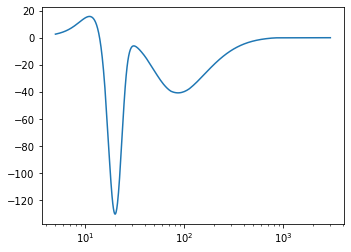
The main results are stored in the attribute sim.history, which is a dictionary containing the evolution of many quantities with time (see the fields listing) for more information on what’s available). To look at the results, you can access these quantities directly:

pl.semilogx(sim.history['z'], sim.history['dTb'])

[<matplotlib.lines.Line2D at 0x185bded90>]

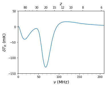
Or, you can access convenience routines within the analysis class, which is inherited by the ares.simulations.Global21cm class:

sim.GlobalSignature(fig=2)

(<AxesSubplot:xlabel='$\\nu \\ (\\mathrm{MHz})$', ylabel='$\\delta T_b \\ (\\mathrm{mK})$'>,
 <AxesSubplot:label='b3e5996d-4a8a-492c-a757-4d11e3b1d6ff', xlabel='$z$'>)

If you’d like to save the results to disk, do something like:

sim.save('test_21cm', clobber=True)

Writing test_21cm.blobs.pkl...
Wrote test_21cm.history.pkl
Writing test_21cm.parameters.pkl...

which saves the contents of sim.history at all time snapshots to the file test_21cm.history.pkl and the parameters used in the model in test_21cm.parameters.pkl.

NOTE: The default format for output files is pkl, though ASCII (e.g., .txt or .dat), .npz, and .hdf5 are also supported. Use the optional keyword argument suffix.

If you just want the plot, you can do, e.g.,

pl.figure(2)
pl.savefig('ares_gs_default.png')

<Figure size 432x288 with 0 Axes>

To read results from disk, you can supply a filename prefix to ares.analysis.Global21cm rather than a ares.simulations.Global21cm instance if you’d like, e.g.,

anl = ares.analysis.Global21cm('test_21cm')

See built-in analysis routines for other options.

See the parameters list to learn about other parameters that can be supplied to ares.simulations.Global21cm as keyword arguments.

2-D Parameter Study

To do simple parameter study, you could do something like:

ax = None
for i, fX in enumerate([0.1, 1.]):
    for j, fstar in enumerate([0.1, 0.5]):
        sim = ares.simulations.Global21cm(fX=fX, fstar=fstar,
            verbose=False, progress_bar=False)
        sim.run()


        # Plot the global signal
        ax, zax = sim.GlobalSignature(ax=ax, fig=3, z_ax=i==j==0,
            label=r'$f_X=%.2g, f_{\ast}=%.2g$' % (fX, fstar))


ax.legend(loc='lower right', fontsize=14)

<matplotlib.legend.Legend at 0x18d149a90>

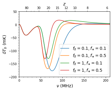
These parameters, along with Tmin, Nlw, and Nion round out the simplest parameterization of the signal (that I’m aware of) that’s tied to cosmology/galaxy formation in any way. It’s of course highly simplified, in that it treats galaxies in a very average sense. For more sophisticated models, check out this example.

Check out the listing of the most common parameters that govern the properties of source populations, and ` <example_grid>`__ for examples of how to run and analyze large grids of models more easily. The key advantage of using the built-in model grid runner is having ARES automatically store any information from each calculation that you deem desirable, and store it in a format amenable to the built-in analysis routines.

A Note About Backward Compatibility

The models shown in this section are no longer the “best” models in ARES, though they may suffice depending on your interests. As alluded to at the end of the previous section, the chief shortcoming of these models is that their parameters are essentially averages over the entire galaxy population, when in reality galaxy properties are known to vary with mass and many other properties.

This was the motivation behind our paper in 2017, in which we generalized the star formation efficiency to be a function of halo mass and time, and moved to using stellar population synthesis models to determine the UV emissivity of galaxies, rather than choosing \(N_{\mathrm{LW}}\), \(N_{\mathrm{ion}}\), etc. by hand (see More Realistic Galaxy Populations). These updates led to a new parameter-naming convention in which all population-specific parameters were given a pop_ prefix. So, in place of Nlw, Nion, fX, now one should set pop_rad_yield in a particular band (defined by pop_Emin and pop_Emax). See the parameter listing for populations for more information about that.

Currently, in order to ensure backward compatibility at some level, ARES will automatically recognize the parameters used above and change them to pop_rad_yield etc. following the new convention. This means that there are three different values of pop_rad_yield: one for the soft UV (non-ionizing) photons (related to Nlw), one for the Lyman continuum photons (related to Nion), and one for X-rays (related to fX). This division was put in place because these three wavelength regimes affect the 21-cm background in different ways.

In order to differentiate sources of radiation in different bands, we now must add a population identification number to pop_* parameters. Right now, fX, Nion, Nlw, Tmin, and fstar will automatically be updated in the following way:

• The value of Nlw is assigned to pop_rad_yield{0}, and pop_Emin{0} and pop_Emax{0} are set to 10.2 and 13.6, respectively.
• The value of fX is multiplied by cX (generally \(2.6 \times 10^{39} \ \mathrm{erg} \ \mathrm{s}^{-1} \ (M_{\odot} \ \mathrm{yr}^{-1})^{-1})\) and assigned to pop_rad_yield{1}, and pop_Emin{1} and pop_Emax{1} are set to 200 and 30000, respectively.
• The value of Nion is assigned to pop_rad_yield{2}, and pop_Emin{2} and pop_Emax{2} are set to 13.6 and 24.6, respectively.
• pop_Tmin{0}, pop_Tmin{1}, and pop_Tmin{2} are all set to the value of Tmin. Likewise for fstar.

Unfortunately not all parameters will be automatically converted in this way. If you get an error message about an “orphan parameter,” this means you have supplied a pop_ parameter without an ID number, and so ARES doesn’t know which population is meant to respond to your change. This is an easy mistake to make, especially when working with parameters like Nlw, Nion etc., because ARES is automatically converting them to pop_* parameters.